Finding the optimal dating strategy for 2019 with probability theory
How knowing some Statistical theory may make finding Mr. Right slightly easier?

Let me start with something most would agree: Dating is hard !!!
(If you don’t agree, that’s awesome!!! You probably don’t spend that much time reading and writing Medium posts like me T — T)
Nowadays, we spend countless hours every week clicking through profiles and messaging people we find attractive on Tinder or Subtle Asian Dating.
And when you finally ‘get it’, you know how to take the perfect selfies for your Tinder’s profile and you have no trouble inviting that cute girl in your Korean class to dinner, you would think that it shouldn’t be hard to find Mr/Mrs. Perfect to settle down. Nope!!! Many of us just can’t find the right match.
Well, I just look, average. In actual fact, if we only look at the data of those who are 168cm in height (imagine a verticle line that goes at 168cm and passes through the red point), I sort of weight a little bit less than these people.
Another important observation is that the plot suggest a positive linear relationship between the height and weight of Vietnamese male. We will do a quantitative analysis to get to the bottom of this relationship.
Dating is far too complex, scary and difficult for mere mortals !!!

Do social media and online dating apps make it easier to find The One? Image Source: Dispatch Weekly
Are our expectations too high? Are we too selfish? Or we simply destined to not meeting The One? Don’t worry! It’s not your fault. You just have not done your math.
How many people should you date before you start settling for something a bit more serious?
It’s a tricky question, so we have to turn to the mathematics and statisticians. And they have an answer: 37%.
What does that mean?
It means out of all the people you could possibly date, let’s say you foresee yourself dating 100 people in the next 10 years (more like 10 for me but that’s another discussion), you should see about the first 37% or 37 people, and then settle for the first person after that who’s better than the ones you saw before (or wait for the very last one if such a person doesn’t turn up)
How do they get to this number? Let’s dig up some Math.
1. The naive (or the desperate) approach:
Let’s say we foresee \(N\) potential people who will come to our life sequentially and they are ranked according to some ‘matching/best-partner statistics’. Of course, you want to end up with the person who ranks 1st — let’s call this person \(X\).
Before we explore the optimal dating policy, let’s start with a simple approach. What if you are so desperate to get matched on Tinder or to get dates that you decide to settle/marry the first person that comes along? What is the chance of this person being \(X\)?

If you can rank these N people. How can you find \(X\)?
Well, it's \(\frac{1}{N}\)
And as \(N\) gets larger the larger timeframe we consider, this probability will tend to zero. Alright, you probably will not date 10,000 people in 20 years but even the small odds of 1/100 is enough to make me feel that this is not a great dating policy.
So what should we do?
We do what people actually do in dating. That is, instead of committing to the first option that comes along, we want to meet a couple of potential partners, explore the quality of our dating fields and start to settle down. So there’s an exploring part and a settling-down part to this dating game.
But how long should we explore and wait?
To formularize the strategy: you date \(M\) out of \(N\) people, reject all of them and immediately settle with the next person who is better than all you have seen so far. Our task is to find the optimal value of \(M\). As I said earlier, the optimal rule value of M is \(M = 0.37N\). But how do we get to this number?
2. A small simulation:
I decide to run a small simulation in R to see if there’s an indication of an optimal value of M.
The set up is simple and the code is as follows:
 # a util function to simulate the 'best-partner rank'
perm_rank <- function(){
  return (sample(1:100, 100))
}

#for each value of M, we simulate 1000 times
M_range <- 2:100, niter <- 1000
# declare a vector to store results, notice that if M = 1, the probability is 1/100
prob_result <- rep(1/100, 100)

# do a simulation for each value of M
for (M in M_range){
  result <- rep(0, niter)
  for (i in 1:niter){
    order <- perm_rank() #simulate the order
    highest_reject <- min(head(order, M-1)) # find the best among the first M-1 that gets rejected
    if (highest_reject != 1){
      accept <- order[order < highest_reject][1]
      # we consider ourselves successful if:
      # - rank 1 is not included in the first M-1 candidates
      # - rank 1 is the first person who is better than all we have seen
      if (accept == 1) result[i] <- 1
      }
  }
  prob_result[M] <- mean(result)
}
We can plot our simulated results for basic visualization:
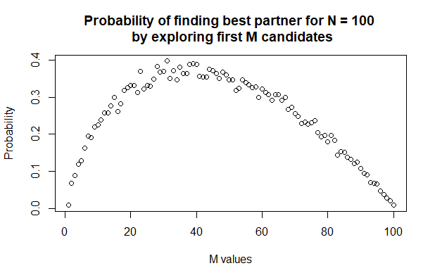
So it seems that with \(N = 100\), the graph does indicate a value of M that would maximize the probability that we find the best partner using our strategy. The value is \(M = 35\) with a probability of 39.4%, quite close to the magic value I said earlier, which is \(M = 37\).
This simulated experiment also shows that the larger the value of \(N\) we consider, the closer we get to the magic number. Below is a graph that shows the optimal ratio \(\frac{M}{N}\) as we increase the number of candidates we consider.
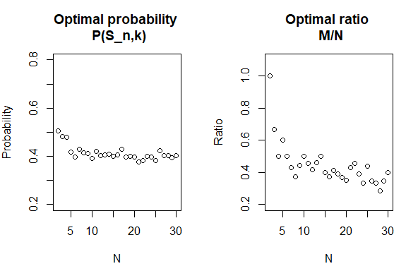
There are some interesting observations here: as we increase the number of candidates \(N\) that we consider, not only does the optimal probability decreases and see to converge, so does the optimal ratio \(\frac{M}{N}\). Later on, we will prove rigorously that the two optimal entities converge to the same value of roughly 0.37.
You may wonder: “Hang on a minute, won’t I achieve the highest probability of finding the best person at a very small value of \(N\)?” That’s partially right. Based on the simulation, at \(N = 3\), we can achieve the probability of success of up to 66% by simply choosing the third person every time. So does that mean we should always aim to date at most 3 people and settle on the third?
Well, you could. The problem is that this strategy will only maximize the chance of finding the best among these 3 people, which, for some cases, is enough. But most of us probably want to consider a wider range of option than the first 3 viable options that enter our life. This is essentially the same reason why we are encouraged to go on multiple dates when we are young: to find out the type of people we attract and are attracted to, to gain some good understanding of dating and living with a partner, and to learn more about ourselves along the process.
You may find more optimism in the fact that as we increase the range of our dating life with N, the optimal probability of finding Mr/Mrs. Perfect does not decay to zero. As long as we stick to our strategy, we can prove a threshold exists below which the optimal probability cannot fall. Our next task is to prove the optimality of our strategy and find that minimum threshold.
Can we prove the 37% optimal rule rigorously?
3. The actual math:
Let \(O_{best}\) be the arrival order of the best candidate (Mr/Mrs. Perfect, The One, X, the candidate whose rank is 1, etc.) We do not know when this person will arrive in our life, but we know for sure that out of the next, pre-determined \(N\) people we will see, \(X\) will arrive at order \(O_{best} = i\).
Let \(S_{n,k})\) be the event of success in choosing \(X\) among \(N\) candidates with our strategy for \(M = k\), that is, exploring and categorically rejecting the first \(k-1\) candidates, then settling with the first person whose rank is better than all you have seen so far. We can see that:
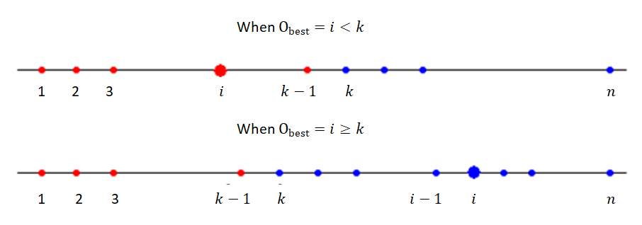
$$P(S_{n,k}|O_{best} = i) = \begin{cases} 0 & i\in \{1,2,3..., k-1\} \\ \frac{k-1}{i-1} & i\in \{k, k+1, ..., n\} \end{cases}$$Why is it the case? It is obvious that if \(X\) is among the first \(k-1\) people who enter our life, then no matter who we choose afterward, we cannot possibly pick \(X\) (as we include \(X\) in those who we categorically reject). Otherwise, in the second case, we notice that our strategy can only succeed if one of the first \(k-1\) people is the best among the first \(i-1\) people.
The visual lines below will help clarify the 2 scenarios above:
Then, we can use the Law of Total Probability to find the marginal probability of success \(P(S_{n,k})\)
$$\begin{array} {lcl} P(S_{n,k}) & = & \sum_{i=1}^{n} P(S_{n,k}|O_{best} = i) \times P(O_{best} = i)\\ &=& \sum_{i=1}^{k-1} 0 \times P(O_{best} = i) + \sum_{i=k}^{n} \frac{k-1}{i-1} \times P(O_{best} = i)\\ &=& \sum_{i=k}^{n} \frac{k-1}{i-1} \times \frac{1}{n}\\ &=& \frac{k-1}{n} \sum_{i=k}^{n} \frac{1}{i-1}\end{array}$$In summary, we arrive at the general formula for the probability of success as follows:
$$P(S_{n,k}) = \begin{cases} 1 & k = 1 \\ \frac{k-1}{n}\sum_{i=k}^{n}\frac{1}{i-1} & k\in \{2, 3, 4, ..., n\} \end{cases}$$We can plug \(n = 100\) and overlay this line on top of our simulated results to compare:
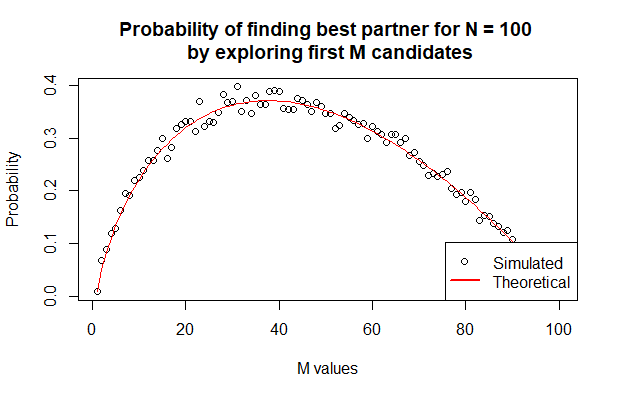
Our theoretical results align perfectly well with the simulated experiment. The theoretical result yields a maximum probability of 37.1% at \(M = 37\)
I don’t want to bore you with more Maths but basically, as n gets very large, we can write our expression for \(P(S_{n,k})\) as a Riemann sum and simplify as follows:
$$P(S_{n,k}) \longrightarrow x\int_{x}^{1} \frac{1}{t} dt = -x\text{ln}(x) $$where \(x= \frac{k}{n}\)
The final step is to find the value of \(x\) that maximizes this expression. Here comes some high school calculus:
$$\frac{d}{dx}(-x\text{ln}(x)) = -\text{ln}(x) - 1$$This derivative has value 0 when \(\text{ln}(x) = -1\) or \(x=e^{-1} \approx 0.3678\)
$$\frac{d}{dx}(-x\text{ln}(x)) = -\text{ln}(x) - 1$$Moreover, at \(x=e^{-1}\):
$$P(S_{n,k}) = -x\text{ln}(x) = e^{-1} \approx 0.3678$$We just rigorously proved the 37% optimal dating strategy.
4. The final words:
So what’s the final punchline? Should you use this strategy to find your lifelong partner? Does it mean you should swipe left on the first 37 attractive profiles on Tinder before or put the 37 guys who slide into your DMs on ‘seen’?
Well, It’s up to you to decide.
The model provides the optimal solution assuming that you set strict dating rules for yourself: you have to set a specific number of candidates \(N\), you have to come up with a ranking system that guarantees no tie (The idea of ranking people does not sit well with many), and once you reject somebody, you never consider them viable dating option again.
Obviously, real-life dating is a lot messier.
Sadly, not everybody is there for you to accept or reject — \(X\), when you meet them, might actually reject you! In real-life people do sometimes go back to someone they have previously rejected, which our model doesn’t allow. It’s hard to compare people on the basis of a date, let alone coming up with a statistic that effectively predicts how great a potential spouse a person would be and rank them accordingly. And we haven’t addressed the biggest problem of them all: that it’s merely impossible to estimate the total number of viable dating options \(N\). If I imagine myself spending most of my time chunking codes and writing Medium article about dating in 20 years, how vibrant my social life will be? Will I ever get close to dating 10, 50 or 100 people?
Another interesting spin-off is to consider what the optimal strategy would be if you believe that the best option will never be available to you, under which circumstance you try to maximize the chance that you end up with at least the second-best, third-best, etc. These considerations belong to a general problem called ‘the postdoc problem’, which has a similar set-up to our dating problem and assume that the best student will go to Harvard (Yale, duh!!!) [1]
The entire Python script for this article can be found at my Github page.
[1] Robert J. Vanderbei (1980). The Optimal Choice of a Subset of a Population. Mathematics of Operations Research. 5 (4): 481–486