The story of the tiny Asian man - How Bayesian statistics convince me to finally hit the gym
"You need to eat more! For a person of your height, you look really skinny"
"Dude! Hit the gymn and your physique will get a lot better"
From high school to college, I often heard people making fun of how small I look, how underweight I must be and how I should do exercise, hit the gym and gain weight in order to have "a nicer physique". I often took these comments with a pinch of salt. For somebody who is 1m69 (5'6) in height and 58kg (127lb) in weight, I have close-to-perfect BMI index (20.3).
I don't look quite like this but you get the idea. Image source: Clip Art Library
"No dude! We are talking about the physique"
Ok, I get it, nobody is talking about BMI here. Thinking about it, people may have a good point: given that I am slightly taller and have the exact same weight as an average Vietnamese male (a Wikipedia profile of 1m62 and 58kg), I may "look" a little skinnier. Look is the key word here. The logic is quite simple, isn't it? If you stretch yourself a little bit and have the same exact weight, you should look, well, leaner and skinnier. Nonetheless, this is actually serious scientific question to investigate further: How small I am (in weight) for a Vietnamese male of 1m69 in height?
We need a methodological way to investigate into this topic. A good way to go forward is to find as much data of Vietnamese men's height and weight as possible and see where I stand among them.
After browsing through the web, I found out a survey research data1 that contains demographic information of more than 10,000 Vietnamese people. I limited the sample size to Male of the age group 18-29. This allows me to have a sample size of 383 Vietnamese males whose age are around 18-29, which is probably good enough for analysis.
At first, let's plot the data's weight and see how I would fit in among the young Vietnamese men.
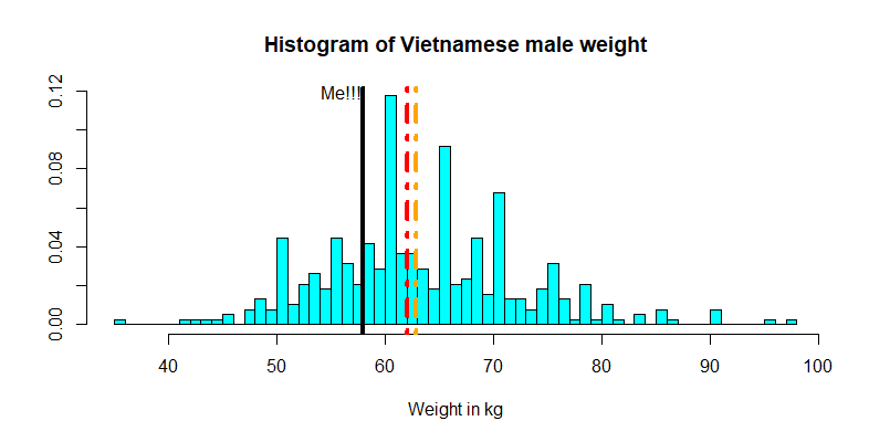
The red line shows the median of the sample while the orange line shows the mean
This plot suggests that I am slightly below both the average and median weights of those 383 Vietnamese young men. Encouraging news? However, the question is not really about how my weight compares to those in this sample per se, but given the height of 1m68 what can we infer about my weight compared to the entire Vietnamese population, assuming that the Vietnamese male population is well-represented by these 383 individuals? To do this, we need to dive into a regression analysis.
At first, let's plot a 2-dimensional scatter plot of heights and weights
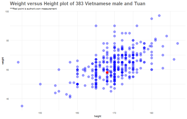
Well, I just look, average. In actual fact, if we only look at the data of those who are 168cm in height (imagine a verticle line that goes at 168cm and passes through the red point), I sort of weight a little bit less than these people.
Another important observation is that the plot suggest a positive linear relationship between the height and weight of Vietnamese male. We will do a quantitative analysis to get to the bottom of this relationship.
First, let's quickly add a "standard least square" line. I will say more about this line later and just show it for now.
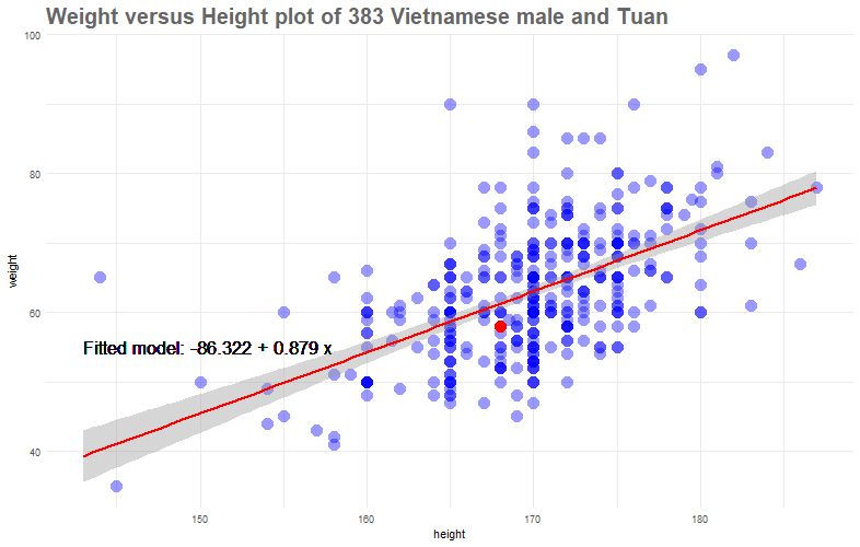
We could interpret our least-squares line \(y = -86.32+0.889x\) as suggesting that the usual profile of a Vietnamese male at my age is such that an increase in 1 cm of height would observe an increase in weight of 0.88kg.
However, this does not answer our question; that is, given somebody of my height (1m68), is 58kg considered too much, too little or just about average? To rephrase this question in a more quantitative manner, if we have a distribution of all of those who are 1m68 in height, what is the chance of my weight falls into the 25,50 or 75-percentile? To do this, let's dig deeper and try to understand the theory behind Regression.
The theory of Linear Regression:
In a linear regression model, the expected value of the \(Y\) variable (in our case, the weight) is a linear function of \(x\) (height). Let’s call the intercept and slope of this linear relationship \(\beta_0\) and \(\beta_1\); that is, we assume that \(E(Y | X = x) = \beta_0 + \beta_1x\). We do not know \(\beta_0\) and \(\beta_1\) so we treat these as unknown parameters.
In the most standard linear regression model, we further assume that the conditional distribution of \(Y\) given \(X = x\) is Normal.
This means that simple linear regression model:
$$Y = \beta_0 +\beta_1x + \epsilon$$can be rewritten as:
\begin{equation} \mu_i = \beta_0 + \beta_1x_i \end{equation} $$y_i \sim N(\mu_i, \sigma)$$Note that in many models, we can replace variance parameter \(\sigma\) with precision parameter \(\tau\), where \(\tau = 1/\sigma\).
To summarize: dependent variable \(Y\) follows normal distribution parametrized by mean \(\mu_i\), that is a linear function of \(X\) parametrized by \(\beta_0\),\(\beta_1\), and by precision parameter \(\tau\).
Finally, it only remains to say what we are assuming about the variance/precision. In particular, we are assuming the unknown variance does not depend on \(x\); this assumption is called homoscedasticity.
That's a lot, but you can visualize what I have discussed with this photo
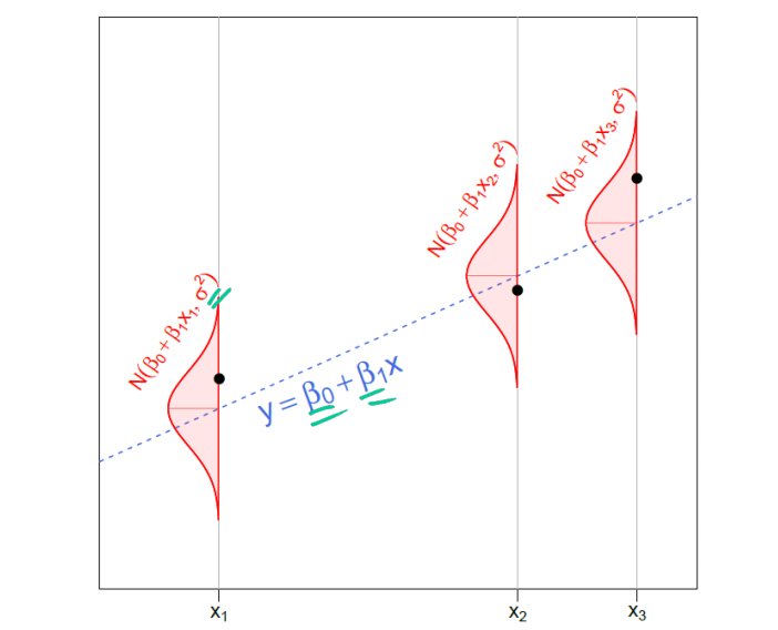
In an actual data analysis problem, all we are given is the black dots—the data. Using the data, our goal is to make inferences about the things we don’t know including \(\beta_0\) and \(\beta_1\) (which determine the shadowy, mysterious, blue dotted line) and \(\sigma\) (which determines the width of the red Normal densities from which the \(y\) data values are drawn).Image source: Joseph Change's Yale S&DS 238 course.
Estimating parameters
Now, there are a couple of ways you can do to estimate \(\beta_0\) and \(\beta_1\).If you estimate such model using ordinary least squares, you do not have to worry about the probabilistic formulation, because you are searching for optimal values of \(\beta_0\) and \(\beta_1\) by minimizing the squared errors of fitted values to predicted values. On another hand, you could estimate such model using maximum likelihood estimation, where you would be looking for optimal values of parameters by maximizing the likelihood function
$$\mathop{\arg\,\max}\limits_{\beta_0, \beta_1, \tau} = \prod_{i=1}^{n} N(y_i;\beta_0 + \beta_1x_i, \tau) $$Note: an interesting result (not demonstrated mathematically here) is that if we make the further assumption that the errors belong to a normal distribution the least squares estimators are also the maximum likelihood estimators.
Linear Regression with a Bayesian touch:
The Bayesian approach, instead of maximizing the likelihood function alone, would assume prior distributions for the parameters and use Bayes theorem:
$$posterior \propto prior\times likelihood$$The likelihood function is the same as above, but what changes is that you assume some prior distributions for the estimated parameters \(\beta_0\), \(\beta_1\), \(\tau\) and include them into the equation:
\begin{equation} f(\beta_0, \beta_1, \tau) \propto \prod_{i=1}^{n}N(y_i;\beta_0 + \beta_1x_i, \tau)f_{\beta_0}(\beta_0)f_{\beta_1}(\beta_1)f_{\tau}(\tau) \end{equation}Now, this prior business feels kind of strange. The truth is, there is a very strong philosophical reasoning as to why we could assign an unknown parameters (in our case \(\beta_0\), \(\beta_1\), \(\tau\) ) with some seemingly arbitrary distributions. These prior distributions are meant to capture our beliefs about the situation before seeing the data. After observing some data, we apply Bayes' Rule to obtain a posterior distribution for these unknowns, which takes account of both the prior and the data. From this posterior distribution we can compute predictive distributions for future observations.
The final estimate will depend on the information that comes from your data and from your priors, but the more information is contained in your data, the less influential are priors.
"What distributions?" is a different question, since there is unlimited number of choices. There is (in theory) just one correct prior, the one that captures your (subjective) prior beliefs. However, in practice, the choice of the prior distribution can be rather subjective and sometimes, arbitrary. We could just choose a Normal prior with a large standard deviation (small precision); for example, we could assume \(\beta_0\) and \(\beta_1\) come from a Normal distribution with mean 0 and SD 10,000 (precision = \(1 \times 10^{-5}\)) or whatever. This is called an uninformative prior because the distribution will be rather flat (that is, it assign almost equal distribution to any value in a particular range). What follows is that if this type of distribution is our choice, we do not need to worry about which distribution among spread-out distributions might be better because they are all nearly flat in the region where the likelihood is non-negligible, and the posterior distribution doesn’t care what the prior distribution looks like in regions where the likelihood is negligible.
Similarly, for the precision \(\tau\), we know these must be nonnegative so it makes sense to choose a distribution restricted to nonnegative values– for example, we could use an Gamma distribution with low shape and scale paraeter.
Another useful uninformative choice is the uniform distribution. If you choose a uniform distribution for \(\sigma\) or \(\tau\), you may end up with a model that is illustrated by John K. Kruschke
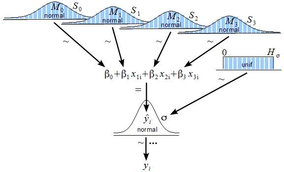
John K. Kruschke's illustrated model. Image source: Indiana University.
JAGS
So far so good for the theory. The issue is that while solving equation (2) is most of the time achievable with derivative optimization, solving equation (3) is mathematically more challenging . In vast majority of cases posterior distribution will not be directly available (see how complicated Normal and Gamma distribution is and you have to MULTIPLY a series of those together). Markov Chain Monte Carlo methods is often used for estimating the parameters of the model. JAGS helps us does exactly that.
The idea behind JAGS model is that a simulation process based on Markov Chain Monte Carlo will generate many iterations of parameter space \(\theta = (\beta_0; \beta_1; \tau)\). The distribution of the sample generated for each parameter in this parameter space will approximate (proven mathematically) the population distribution of the parameter.
We run JAGs in R as follows
- At first, we write our model in text format:
 n <- 383 #number of observation

 mymodel <- "
 model{
  for(i in 1:n){
    # set up our model
    y[i] ~ dnorm(a + b*x[i], tau)
  }
  # state our prior distribution
  # JAGs requires that we use precision
  # not variance in linear model
  a ~ dnorm(0, 1e-6)
  b ~ dnorm(0, 1e-6)
  tau ~ dgamma(.01,.01)
  }"
Then, we command JAGs to conduct the simulation. Here I ask JAGs to simulate the value for the parameter space \(\theta\) 10000 times.
 jm <- jags.model(file = textConnection(mymodel), data=list(n=n, x=data$height, y=data$weight))
 cs <- coda.samples(jm, c("a","b","tau"), 10000)
 sample_data <- as.data.frame(cs[[1]])
After such sampling, we achieve the sampled data of \(\theta = (\beta_0; \beta_1; \tau)\) such as this
| \(\beta_0\) | \(\beta_1\) | \(\tau\) | |
|---|---|---|---|
| 1 | -66.30087 | 0.7654910 | 0.01500597 |
| 2 | -66.97430 | 0.7623432 | 0.01610994 |
| 3 | -66.88992 | 0.7537466 | 0.01793836 |
| 4 | -66.09944 | 0.7537466 | 0.01644814 |
Great, now we have 10,000 iterations of the parameter space \(\theta\), what do we do now? Remember that by equation (1):
$$\mu = \beta_0 + \beta_1x$$This means that if we substitute \(x = 168cm\) to each of the iteration, we will find 10,000 values of weight and thus, the distribution of weights given that the height is 168cm.
cmean <- sample_data$a + sample_data$b*168
We are interested in the percentile of my weight, conditional on my height. For any quantity that can be calculated as a function of the parameters we have monitored in the MCMC, we can get a sample from the posterior distribution for that quantity simply by taking that function of the parameters in our MCMC. We’ll do that for the desired percentile here.
  m_perc <- pnorm(q = m_weight, mean = cmean, sd = sample_data$sig)
 truehist(m_perc)
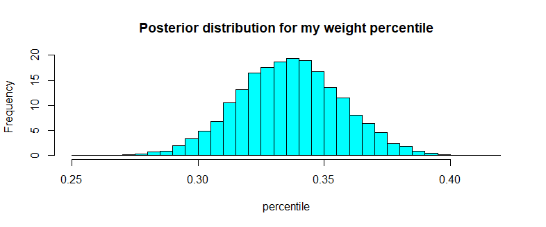
Oophs!!! I will not even be in the range.
For example, we can find the percentile that my weight is in the first 40 percentile or less
  mean(m_perc <= 0.4)
 #  [1]  0.994
So there is overwhelming evidence that conditional on my height of 168cm, my weight 58kg would leave me at the lower percentile of the Vietnamese population. Much as I hesitate to admit, I am indeed very skinny for somebody of 168cm in height. It's really about time to hit the gym and gain some weights. After all, if you cannot trust some well done Bayesian statistics result, what else can you trust?
Update: I have included in the data source a dataset that that contains the height and weight of 8169 male and female youth in America (National Longitudinal survey 19972), could you conduct the same analysis and see where you stand?
The entire Python script for this article can be found at my Github page.
Data Source: Vuong Q. H.. Open Science Framework. 2017 https://doi.org/10.17605/OSF.IO/AFZ2W
Data Source: National Longitudinal Surveys | Bureau of Labor Statistics 1997 https://www.nlsinfo.org/investigator/pages/search.jsp?s=NLSY97